The MathMap Language Tutorial
MathMap is a language for transforming existing images and
producing entirely new ones. Think of it as the ultimate image and
animation filter. This flexibility, however, comes at a price: Using
MathMap to create a new transformation isn't as simple as using some
pre-built image manipulation filter. Instead, you have to precisely
describe what MathMap should do. This usually requires a bit of math
knowledge (for most tasks, high-school math is more than sufficient)
and it is necessary to know the MathMap language.
This document is a gentle introduction to the
MathMap language. Very little mathematical knowledge is assumed, and
almost no programming skills are needed--although they would certainly
come in handy.
Please take the time to read through this introduction. Try out
the examples we give and play around with them. Change them a little
and see what happens. That way, you will quickly gain a feeling for
what you can achieve with MathMap and in which ways. If you do this,
we are confident that you will soon create your own image filters and
maybe even get hooked on MathMap.
This tutorial deals with the following topics:
Basic Principles
The Cartesian Coordinate System
Input Images
The Polar Coordinate System
Conditionals
Variables
User Values
Animations
Basic Principles
The basic operating principle of MathMap is very simple. To create
an image of a given size, MathMap simply goes through all the
elements (pixels) of the image to be created and "asks" your filter
how the pixel in question should look like, i.e. what color it should
have.
Let's make a filter that produces a white image:
filter white ()
    grayColor(1)
end
As you can see, MathMap filters always start with the word
filter and end with the word end. The word
white after filter is simply the name of the filter
and you are free to choose your own names as you like. The
parentheses () serve a purpose which we'll come to later.
grayColor is a function producing a gray level color.
What it needs to know is the gray level you want to produce. In this
case, the gray level we want is 1, which stands for white.
0 is black, and 0.5 is halfway in between. If you
provide a value greater than 1, MathMap will use 1
instead (there is no color whiter than white!). Similarly, 0
will be used if a value less than 0 is passed to the
function.
Such values given to functions are called arguments. As
we have just seen, grayColor takes exactly one
argument. Arguments are always given to a function after its name,
enclosed in parentheses. As we will shortly see, if a function takes
more than one argument, those arguments are separated by commas.
Producing gray levels is fun, but we'd like to play around with
"real" colors, too. So, let's produce a red image:
filter red ()
    rgbColor(1, 0, 0)
end
As you can see, rgbColor takes three arguments and
produces a color. Its first argument is the amount of red in the
color. The second argument is the color's green component, and the
third argument specifies the blue component. Again, useful values
range from 0 to 1. Values too large
or too small are clipped to 1 or 0, respectively.
Try to change the values and see how it affects the output color.
The Cartesian Coordinate System
So far, the pixels in our images have always had the same color. When
we produce images with multiple colors, we usually want to determine
the color based on the position of the pixel in question.
MathMap allows access to the coordinates of the pixel being
calculated. It supports two coordinate systems. The first one, which
you are certainly familiar with, is the cartesian coordinate system.
Each pixel has two coordinates, called x and
y. The following figure illustrates the cartesian coordinate
system:
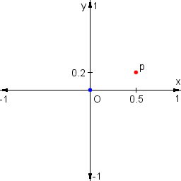
The point labeled "O" is the origin of the coordinate
system. Both its coordinates (x and y) are zero.
The origin is always in the center of the image. The point "p" in the
illustration has a value of 0.5 for the coordinate x
and 0.2 for y. That's because it's halfway from the
origin to the right edge of the image and one fifth to the top edge.
As you can see, the x coordinate is 1 at the right
edge of the image and -1 at the left edge. The same holds
for the y coordinate and the top and bottom edges,
respectively.
Let's use this knowledge to produce an image which is black on the
left, white on the right and has gray levels in between. We want to
produce this image:

We know that we can use grayColor to produce a gray level.
However, we need a number between 0 and 1 to get
colors between black and white. Let's look at what we have. At the
right edge of the image the value of x is 1 and at
the left edge it's -1. In order to get 0 at the
left edge, we can simply add 1 to x,
i.e. use x+1. At the right edge, however, we now
get 2 instead of 1, which we can rectify by dividing
by 2, which gives us (x+1)/2. Now we have what we
want, and we can give this expression as an argument to
grayColor:
filter gray_gradient ()
    grayColor((x + 1) / 2)
end
Try to do the same for the y coordinate, i.e. make a
gradient from bottom to top instead of from left to right. You could
also try to combine both coordinates to produce a gradient which goes
from the bottom left corner to the top right corner.
Input Images
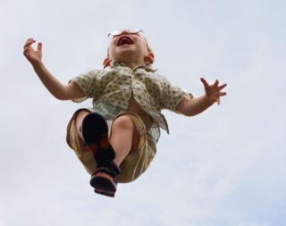
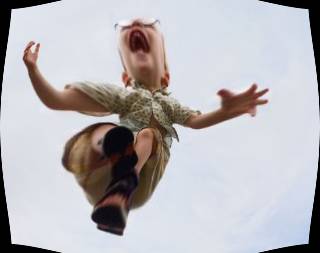
While it's fun to produce completely new images, it is often nice
or necessary to modify existing ones. We will use this as our input
image:
What we have to do is tell MathMap that we want to give it an input
image, and we have to give it a name, because there might be more than
one. That's where the parentheses after the name of the filter come
in. Between them, we give all the inputs our filter gets:
filter ident (image in)
    in(xy)
end
A few things are new here. Notice the declaration of the input
image, which we call in. The reason why we have to specify
with the word image that it's an image is that there are
input types other than images, which we'll come to later.
What's new as well is the way we use the input image. It looks
exactly like using a function with one argument, in this case
xy, which we haven't explained yet, either. xy is a
variable that combines x and y in one value, with
the additional information that it's cartesian coordinates. That
information is necessary because, as we'll see later, MathMap supports
another coordinate system, as well.
So, you can use an input image just like you use a function. It
takes one argument, namely the coordinates of the pixel that you
request. In the script above, we are simply passing along the
coordinates that our filter is given, so we just copy the input image,
which is not very exciting.
A very simple effect is to flip the image horizontally. This can
be achieved by changing the sign of the x coordinate,
i.e. making negative coordinates positive and vice versa:
filter flip (image in)
    in(xy:[-x, y])
end
There's two other new pieces of syntax here. First of all we're
using square brackets to combine the x and y coordinates into one
value, called a "tuple". You can build tuples with as many numbers as
you like. Tuples can only contain numbers, though, and not other
tuples. The variable xy that we've seen in the filter
ident above is a tuple, as well.
In addition, we're using the colon to give the tuple a so-called
"tag", namely xy, which actually has no direct relation to
the variable xy seen above. This specific tag says that the
tuple is a pair of cartesian coordinates. Without that tag, MathMap
wouldn't know which coordinate system you're using to request a pixel
from the input image.
Try out the script for yourself. Also, try to predict what would
happen if you changed the sign of the y coordinate instead,
then try it out and see if you were right.
Now, let's shake the waves with our image. The function
sin will come in handy for our purposes. This is what its
graph looks like (by the way, this graph was produced by MathMap,
using an expression by Hans Lundmark):
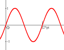
As you can see, the value of sin oscillates
between -1 and 1. The length of its oscillation
period (the distance it needs to make a whole "cycle") is
2*pi. The value of pi, as is well known, is about
3.14159.
We will now try to shift whole pixel columns up and down, depending
on their x coordinates. The shift pattern will resemble the
graph of the sin function, only that we will use a period
length of half the width of the image, i.e. 1, and we will
shift them up or down by at most 0.1:
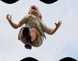
filter sine_finn (image in)
    in(xy:[x, y + 0.1 * sin(x * (2*pi))])
end
The resulting image looks like this:
The Polar Coordinate System
In addition to the familiar cartesian coordinate system, MathMap
also supports the polar coordinate system. Each pixel has two polar
coordinates, namely r and a. The
following illustration helps in understanding the polar coordinate
system:
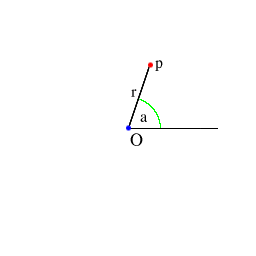
The value of r is simply the distance from the origin
(i.e. the center of the image) to that pixel.
The value of a is the angle between the positive x-axis
and the line from the origin to the pixel in question.
However, the angle is not measured in degrees
(0-360), but in radians, which range from 0
to 2*pi. This may seem a bit awkward, but it is more
convenient mathematically. MathMap provides two functions to
convert between radians and degrees, namely rad2deg and
deg2rad.
Polar coordinates make it very easy to generate pond-like effects.
When we try the wavy script from above and use polar instead of
cartesian coordinates, leaving the a coordinate unchanged and
shifting the r coordinate, we get the following expression:
filter finn_pond (image in)
    in(ra:[r + 0.1 * sin(r * (2*pi)), a])
end
which generates this image:
Notice how this script uses the tag ra, instead of
xy, to let MathMap know that the coordinates given to the
input image are polar and not cartesian.
Conditionals
Let's create an image which looks like a shooting target:
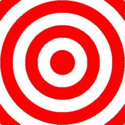
Obviously, whether a pixel is red or white depends solely on its
distance from the center, which we know is available as r. I
have chosen the width of each ring as 0.2, i.e. the distance
between the radii of the inner circles of two neighboring red (or
white) rings is 0.4. Hence, the expression we
are looking for is periodic with a period of 0.4.
To solve this problem, we will use the modulo operator, which is
available as %. Its value is the remainder of the division
of its left operand by its right operand. As an example, 7%3
is 1 because the remainder of the division of
7 by 3 is 1.
This operation is periodic. Its period is the value of its right
operand (the divisor). Furthermore, the result of the operation is
never greater than the right operand. So, for example, r%0.4
is periodic with a period of 0.4 and is always
between 0 (inclusive) and 0.4 (exclusive). Let's see
what this looks like:
filter rmod ()
    grayColor((r%0.4)/0.4)
end
In order to be nice to grayColor, the value
is scaled to be in the range from 0 to 1 (instead of
0.4). The resulting image looks like this:
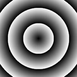
You can see that the value starts out as 0 at the center
of the image, climbs to 1 at a distance of 0.4 from
the center and then immediately drops to 0 again, repeating
this cycle forever (well, in our case, to the boundaries of the
image).
You may want to try to leave out the rescaling "/0.4" to
see the difference.
All we have to do now is to check whether we are in the first half
of a period (in which case r%0.4 is less than 0.2), or
in the second. If we are in the first, the color for the pixel is
red, otherwise it is white. MathMap provides a construct for such
decisions:
filter target ()
    if r%0.4 < 0.2 then
        rgbColor(1,0,0)
    else
        rgbColor(1,1,1)
    end
end
The indentation is used merely to make the expression easier to
read. You can indent your code any way you like (or not at all).
The expression should be easy enough to understand. If the
condition is fulfilled, the result is the color red, otherwise it is
the color white.
Variables
Sometimes you want to use one value in multiple places in your
expression. It's not necessary to write that value twice. Instead
you give it a name by which you can refer to it later. Let's say we
want to produce an image like this:

As you can see, the pixels from the original image fade to black
with the distance from the center. They reach the black color at the
corners of the image.
The variable r, which holds the distance from the center
of the image, is measured in the same distance units as the cartesian
coordinates, and its maximum value, which it reaches in the four
corners of the image, is provided by the constant
R (which is the square root of 2 in square images,
in case you must know). If we scale this down to 1, it's
much easier to work with, so we'll use r/R. This
expression's value is 0 at the center of the image and
increases with the distance from the center. It reaches 1 in
the corners, exactly where we want the color to be solid black.
Given the color of a pixel in the original image and its
transformed (as above) distance from the center, we can now figure out
what to do. If the transformed distance is 0
(in the center) we want the original color unchanged. If it's
1, we want the color black. We can reach that effect by
multiplying the three color components of the pixel by 1
minus the transformed distance, i.e. by 1-r/R.
We can use the functions red, green, and blue
to access the components of a color. Now we could write the red
component of our output image as red(in(xy))*(1-r/R). We'd
have to use equivalent expressions for the green and blue components
and then use them as arguments to rgbColor. By assigning the
values in(xy) and 1-r/R to variables, which we'll
call p and d (you can choose any name you like, as
long as it's not the name of a built-in constant or variable or a
keyword; consult the MathMap reference
for the names of all of those), we can write the resulting expression
much shorter as rgbColor(red(p)*d, green(p)*d, blue(p)*d).
The complete filter is:
filter finn_vignette (image in)
    p=in(xy);
    d=1-r/R;
    rgbColor(red(p)*d, green(p)*d, blue(p)*d)
end
As you can see, assigning values to variables is very
straightforward. You must separate variable assignments and other
expressions with semicolons.
By the way: Using more advanced features of MathMap you can write
an expression equivalent to the above as
filter finn_vignette (image in)
    lerp(r/R, in(xy), grayColor(0))
end
So, please go on reading, there's more to come.
User Values
Sometimes you need to put some values into your script which
are more or less arbitrary. Often you want to try out several
different values, and it's tedious to change the script every time
by hand. That's where user values come in. Let's reiterate our wave
example:
filter sine_finn (image in)
    in(xy:[x, y + 0.1 * sin(x * (2*pi))])
end
There are two parameters here which we have chosen more or less
arbitrarily, namely the amplitude of the wave (in this case
0.1) and the wave length (in this case implicitly given
as 1). Wouldn't it be nice if we could change these values
with sliders instead of having to edit the expression?
That's where inputs come in again. We've seen above that we can
give images as inputs to filters. Now we'll learn how to supply
numbers as well:
filter sine_finn (image in, float amplitude: 0-2, float wavelength: 0-10)
    in(xy:[x, y + amplitude * sin(x * (2*pi) / wavelength)])
end
The type float denotes a so-called floating point
number, which represents a real number and can have a fractional
component, in contrast to integers, which you can specify with the
word int. After the name of the argument you can also give a
range of allowed values, in the case of the argument
amplitude above from 0 to 2.
There are not only argument types for images and numbers, but also
for colors, color gradients and curves. Check out the Reference Manual for details.
Tuples and Tags
Now it's time to look at a more technical subject, namely MathMap's
type system. We've already talked about it a little when we examined
coordinates, and now we'll go into a bit more detail.
The type system of MathMap is designed to be as invisible as
possible, but in order to unleash MathMap's full potential, you will
need to know one or two things about it. Don't worry, it's not very
complicated.
Sometimes it's convenient to treat two or more numbers as a single
value. One such example is colors. A single color is actually four
distinct numbers. We have already come across three of them, namely
the red, green, and blue components. The fourth is the color's
transparency value, called alpha. A color with an alpha of
1 is completely opaque, like all the colors we have seen so
far. An alpha component of 0 means full transparency,
0.5 means half transparent, and so on.
So far, we have always treated colors as single values. We have
constructed colors using functions such as rgbColor and
retrieved their components with functions like red. We can,
however, do these things without using those functions. This, for
example, is the half-transparent color green:
rgba:[0, 1, 0, 0.5]
One or more numbers within square brackets, separated by commas,
constitute a tuple. So, tuples are just ordered collections
of numbers. They are ordered because MathMap remembers in which order
you have written their components. For example, the tuple
[1,2,3] is not the same as [3,2,1].
The name rgba is a tag. The tag rgba
tells MathMap that that tuple is not just four numbers, but a color
with red, green, blue and alpha components. This begs the question
whether there are other kinds of colors. Actually, there are.
MathMap also supports colors in the so-called HSV color
space. Those colors are given the tag hsva. MathMap
uses the tags to determine how to interpret the numbers in the tuples.
Many operators and functions work on tuples as well as on single
numbers. The functions min and max for example,
calculate the minimum and maximum values for each pair of tuple
elements. To set the red component of an image to 0, for
example, you can use the following script:
filter remove_red (image in)
    min(in(xy), rgba:[0, 1, 1, 1])
end
Animations
MathMap provides the functionality to create animations. To that
end, the language provides a variable called t. For each
single picture in the animation (such pictures are called
frames) t has a different value, depending on the
position of the frame within the whole animation. The first picture
in the image always has t set to 0,
while for the last picture it is set to 1. Actually, the
latter statement isn't always true, as we will discover shortly, but
for the time being, simply assume that it is.
The following script produces an animation which fades from black
to white:
filter black_to_white ()
    grayColor(t)
end
You will often want to produce animations which loop seemlessly,
i.e. which look like one endless animation when looped. For such
animations, make sure that the image with a t
value of 1 looks exactly like the one with a value of
0, like in the following script:
filter black_white_loop ()
    grayColor((sin(t * 2*pi) + 1) / 2)
end
The problem here is that if MathMap would render the first image in
the animation with t as 0 and the
last image with t as 1, you would
have the same frame twice when looping. Therefore, MathMap lets you
choose (in the user interface) whether you would like to create a
periodic (looping) animation or not. If you do, t never
reaches 1 at the end of the animation but stops shortly
before, depending on how many frames you want your animation to have.
For example, for a periodic animation with 10
frames, t takes on the values 0, 0.1,
0.2, ... 0.9.
Hint: One way to make periodic animations is to use periodic
functions like sin, cos or the modulo operator
%.
Some Useful Functions
Here is an overview of some MathMap functions which are very useful
in many situations. This is not a complete function reference. If
you are looking for one, you'll find it in the Reference Manual.
Quite often you find that you have a value which varies within a
given range, but you want the range to be different. Take, for
example the gray gradient:
The variable x varies from -1 to 1
but you want it to be between 0 and 1. In such
cases you can use the scale function. The
expression scale(x, -1, 1, 0, 1) is 0
when x is -1 and 1 when
x is 1. Hence, you can create the
above image with the script
filter gray_gradient ()
    grayColor(scale(x, -1, 1, 0, 1))
end
Suppose we want to produce a gradient from red to green:

We know from above that we can use scale(x, -1, 1, 0, 1)
for a value which is 0 at the left image edge
and 1 at the right edge. lerp does
the rest: it takes two tuples and produces a value which is "in
between" these two values by the same amount as its first argument is
in between 0 and 1. Hence, the gradient above can
be produced by this expression:
filter redgreengradient ()
    lerp(scale(x, -1, 1, 0, 1), rgbColor(1,0,0), rgbColor(0,1,0))
end
The function inintv makes it easy to check whether a value
lies within a given range. inintv has a value
of 1 if the condition is fulfilled, and of 0
otherwise. You can use this as a condition in an if
expression, or as a value in its own right. For example, this
script draws a white ring with an inner radius of 0.4 and
an outer radius of 0.6:
filter ring ()
    grayColor(inintv(r, 0.4, 0.6))
end
Sometimes you have values which you want to lie within a given
range. In case they don't, you simply want them to take on the
largest value within the range, if they are too large, or the smallest
if they are too small.
MathMap often does such operations automatically, for example if
you produce colors with components larger than 1 or smaller
than 0.
If you have to do it yourself, clamp can help you. For
example, clamp(v, [0,0,0], [1,1,1]) restricts every element of
v to be in the range from 0 to 1.
The function rand generates a random number. It takes two
arguments: The minimum and the maximum value of the number to be
generated. This filter, for examples, randomly scatters the
pixels of the input image (but not more than a distance of 0.05 away from their
original location in both directions):
filter scatter (image in)
    in(xy:[x + rand(-0.05,0.05), y + rand(-0.05,0.05)])
end
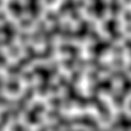
In image manipulation, one often needs a function which is random
but doesn't change as abruptly as rand does. noise
is a so-called solid noise function. It takes a tuple of
three numbers and returns a value between -1 and 1.
If the input arguments change only by a little, so does the resulting
value. The overall "look" of the function is random, though. It's
hard to describe, so it's best you see for yourself:
filter noise_demo ()
    grayColor(scale(noise([x*5, y*5, t*2]), -1, 1, 0, 1))
end
As you can see, the third input value depends on t, so try
out changing t. For t being 0, the
resulting image looks like this:
Further Information
This tutorial has, despite its length, not covered all features and
details of MathMap. For example, we didn't even mention loops (a
programming language feature having nothing to do with animations).
To get more detailed information about the MathMap language, see
the MathMap Reference Manual.
A very good way to learn how to do things with MathMap is to look
at the examples supplied with it. Pick the examples you find
interesting, look at the filter sources, and try to figure out how
they work.
You might also want to look at
the MathMap
Homepage for announcements, new documentation or interesting
links. The best way to get involved in the MathMap community is by
joining the MathMap Google Group.
If you like MathMap, or if you have suggestions or questions
regarding the MathMap language or user interface, feel free to contact the author. I
am looking forward to your feedback.